Annotate equations

👍 Featured as a highlight ✨ in R Weekly 2023-W37 and the R Weekly Podcast 🎧

Annotating Equations

Using the LaTeX annotate-equations package in Quarto allows you to easily annotate equations within your quarto reports, documents or manuscripts. Currently as far as I am aware this only works for pdfs.

Step-by-step example

Here’s a straightforward step-by-step guide to annotating equations using the annotate-equations package. We’ll use the genomic selection GEBV equation as the example.

Quarto Setup

Quarto itself will attempt to automatically download and install the annotate-equations package into its LaTeX engine, all you need to do is tell Quarto that you need it by adding the following to your yaml at the top of your .qmd file

header-includes:
  - \usepackage{annotate-equations}

Begin with Your LaTeX Equation

Start by writing the equation you want to annotate in LaTeX format:

\begin{equation*}
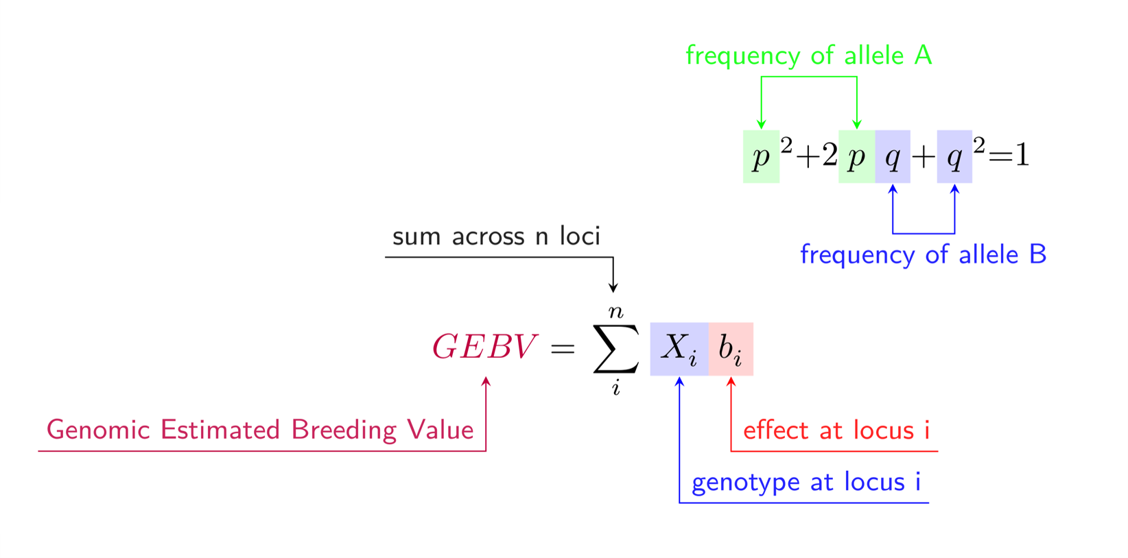
  GEBV = \sum_{i}^{n} X_{i} b_{i}
\end{equation*}

Split the Equation into Nodes

Break down the equation into individual nodes. To highlight a node, enclose it in \eqnmarkbox[color]{node name}{equation term(s)}. If you only want to color the node’s text, use \eqnmark[color]{node name}{equation term(s)}.

For example:

\begin{equation*}
  \eqnmark[purple]{node1}{GEBV}
  \tikzmarknode{node2}{=}
  \eqnmark[black]{node3}{\sum_{i}^{n}}
  \eqnmarkbox[blue]{node4}{X_{i}}
  \eqnmarkbox[red]{node5}{b_{i}}
\end{equation*} 

Add Annotations

Now, introduce annotations to each node using the \annotate[tikzoptions]{annotate keys}{node name[,…]}{annotation text} command:

• For {annotate keys}, choose whether the annotation appears above or below, to the right or left of the node.

• For [tikzoptions], include a yshift value to adjust the annotation’s position above or below (use negative values for below). You may need to fine-tune these values, especially in complex equations. xshift can be defined if necessary.

For example:

\begin{equation*}
  \eqnmark[purple]{node1}{GEBV}
  \tikzmarknode{node2}{=}
  \eqnmark[black]{node3}{\sum_{i}^{n}}
  \eqnmarkbox[blue]{node4}{X_{i}}
  \eqnmarkbox[red]{node5}{b_{i}}
\end{equation*}
\annotate[yshift=1em]{left}{node3}{sum across n loci} 
\annotate[yshift=-1em]{below,left}{node1}{Genomic Estimated Breeding Value} 
\annotate[yshift=-1em]{below,right}{node5}{effect at locus i} 
\annotate[yshift=-2.5em]{below,right}{node4}{genotype at locus i}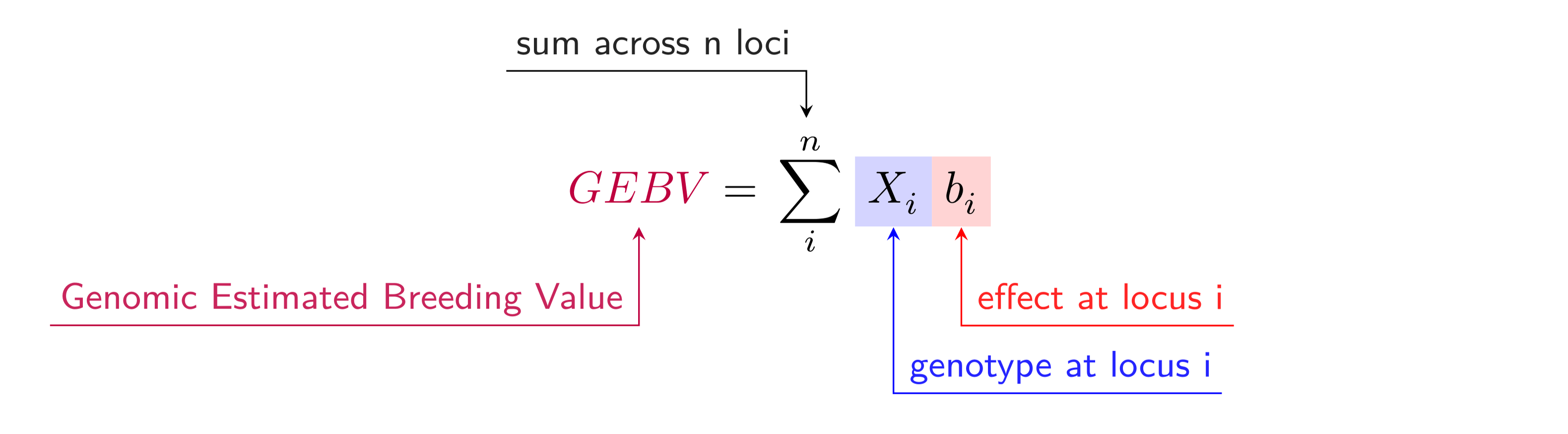

Other example

Annotate to multiple nodes

For some equations a variable will appear multiple times. In these scenarios you may want your annotation to link both occurrences. To archive this you just use the \annotatetwo definition and add both node names.

An example using the Hardy-Weinberg equation:

\begin{equation*}
  \eqnmarkbox[green]{node1}{p}
  \tikzmarknode{node2}{^{2}}
  \tikzmarknode{node3}{+}
  \tikzmarknode{node4}{2}
  \eqnmarkbox[green]{node5}{p}
  \eqnmarkbox[blue]{node6}{q}
  \tikzmarknode{node7}{+}
  \eqnmarkbox[blue]{node8}{q}
  \tikzmarknode{node9}{^{2}}
  \tikzmarknode{node10}{=}
  \tikzmarknode{node11}{1}
\end{equation*}
\annotatetwo[yshift=1.5em]{above, label above}{node1}{node5}{frequency of allele A} 
\annotatetwo[yshift=-1.5em]{below, label below}{node6}{node8}{frequency of allele B} 

Additional Information

If you want to see how this looks in a pdf and/or see the LaTeX code inside the correpsonding quarto .qmd file visit my github repo.

For more in-depth instructions and possibilities with annotate-equations in LaTeX, refer to the documentation at https://github.com/st–/annotate-equations/blob/main/annotate-equations.pdf